This document will get you up to speed on using marquee for rich text formatting in R graphics. Marquee is collectively a markdown dialect, a parser for the dialect and a grid renderer for text written in the dialect. The package aims to fill the same use cases as gridtext and ggtext by Claus Wilke, but works in a very different and more low-level way.
Requirements
Before we start we should note that marquee has been build for the future. What I mean by this is that it is based on a slew of new features in the R graphics engine putting very hard requirements on what R version it can be used with and which graphics devices it works with. If, for some reason, your setup cannot accommodate these needs you can perhaps get some of the way using gridtext/ggtext. The nuisance of this will likely diminish or completely disappear with time.
An example
md_text <-
"# Lorem Ipsum
Lorem ipsum dolor sit amet, *consectetur* adipiscing elit, sed do eiusmod tempor incididunt ut
labore et dolore magna **aliqua**. Ut enim ad minim veniam, quis nostrud exercitation ullamco
laboris nisi ut aliquip ex ea commodo _consequat_. Duis aute irure dolor in reprehenderit in
voluptate velit esse cillum dolore eu fugiat nulla ~pariatur~. Excepteur sint occaecat
cupidatat non proident, sunt in culpa qui officia deserunt mollit anim id est laborum."

grob <- marquee_grob(md_text, classic_style())

grid.draw(grob)
From this small example you can see that markdown behaves as you’d expect. We have emphasis, strong, underline, and strikethrough, and stuff like headings etc. In fact, the full markdown (CommonMark) spec is supported and will behave as you’d expect.
Besides the standard grob arguments you’d expect,
marquee_grob() takes two main arguments as you can see
above. The text, which can be a character vector with multiple separate
markdown strings, and a style specification, which again can be a vector
of styles or a single style to format everything alike. Marquee ships
with classic_style() which is designed to mimic the look of
standard HTML rendered markdown. The function itself allows you to
modify the final style, and you could also modify it after construction
to create a completely new style:
new_style <- classic_style(body_font = "serif", header_font = "mono", hanging = em(1))

new_style <- modify_style(
  new_style,
  "str",
  background = "lightgrey",
  border_radius = 3,
  padding = trbl(em(0.2))
)

grid.draw(
  marquee_grob(md_text, new_style)
)
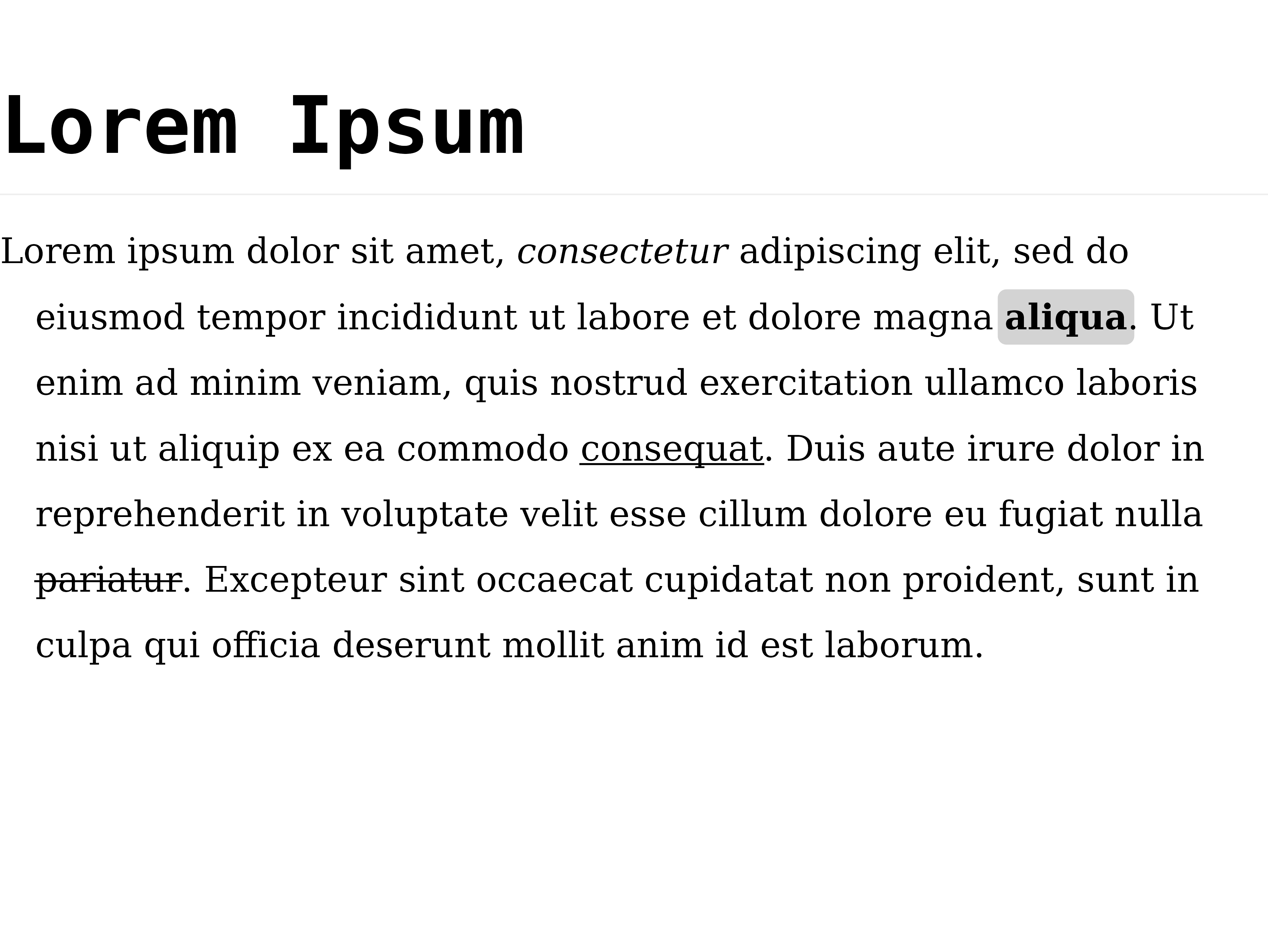
Besides standard markdown, marquee also allows you to create custom span classes. These span classes can be styled to anything, but marquee contains a nifty feature where, if the class matches a recognized color name or hex-code, it will be automatically coloured.
md_text_custom <-
"# Lorem Ipsum
Lorem ipsum dolor {.red sit amet, *consectetur* adipiscing elit, sed do} eiusmod tempor
incididunt ut labore et dolore magna **aliqua**. Ut enim ad minim {#2af veniam}, quis nostrud
exercitation ul lamcolaboris nisi ut aliquip ex ea commodo _consequat_. Duis aute irure dolor
in reprehenderit in voluptate velit esse cillum dolore eu fugiat nulla ~pariatur~. Excepteur
sint occaecat cupidatat non proident, sunt in culpa qui officia deserunt mollit anim id est
laborum."

grid.draw(
  marquee_grob(md_text_custom, classic_style())
)
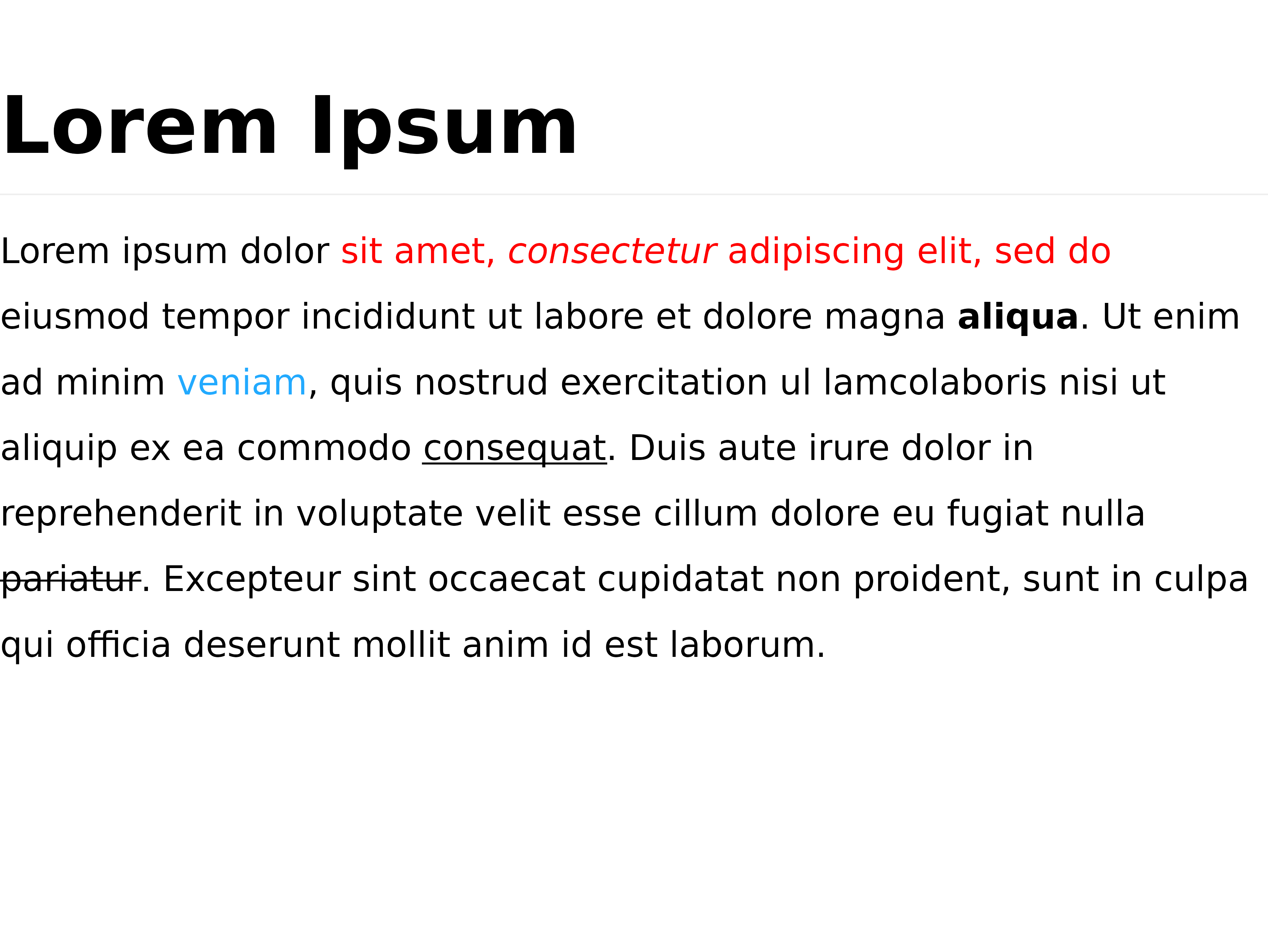
If you provide a styling for the custom class it takes precedence over any matching color name
grid.draw(
  marquee_grob(md_text_custom, modify_style(classic_style(), "red", tracking = 400))
)
Use in ggplot2
Recognizing that most people doesn’t make visualizations directly with grid, marquee also contains the infrastructure to use markdown inside ggplot2 plots. It is expected that these functions will eventually move to ggplot2 proper, but while the package is stress tested they will stay here.
The marquee geom
One way to use marquee with ggplot2 is with
geom_marquee(). It supersedes both geom_text()
and geom_label() in its capabilities, and even if you don’t
need to plot rich text, the styling of geom_marquee() is
much more capable:
fancy_font <- classic_style(
  weight = "semibold",
  features = systemfonts::font_feature(
    ligatures = c("standard", "discretionary"),
    letters = c("stylistic", "swash", "historical")
  )
)
ggplot(mtcars, aes(disp, mpg, label = rownames(mtcars))) +
  geom_marquee(style = fancy_font, size = 2.5, family = "spectral") # You may not have this font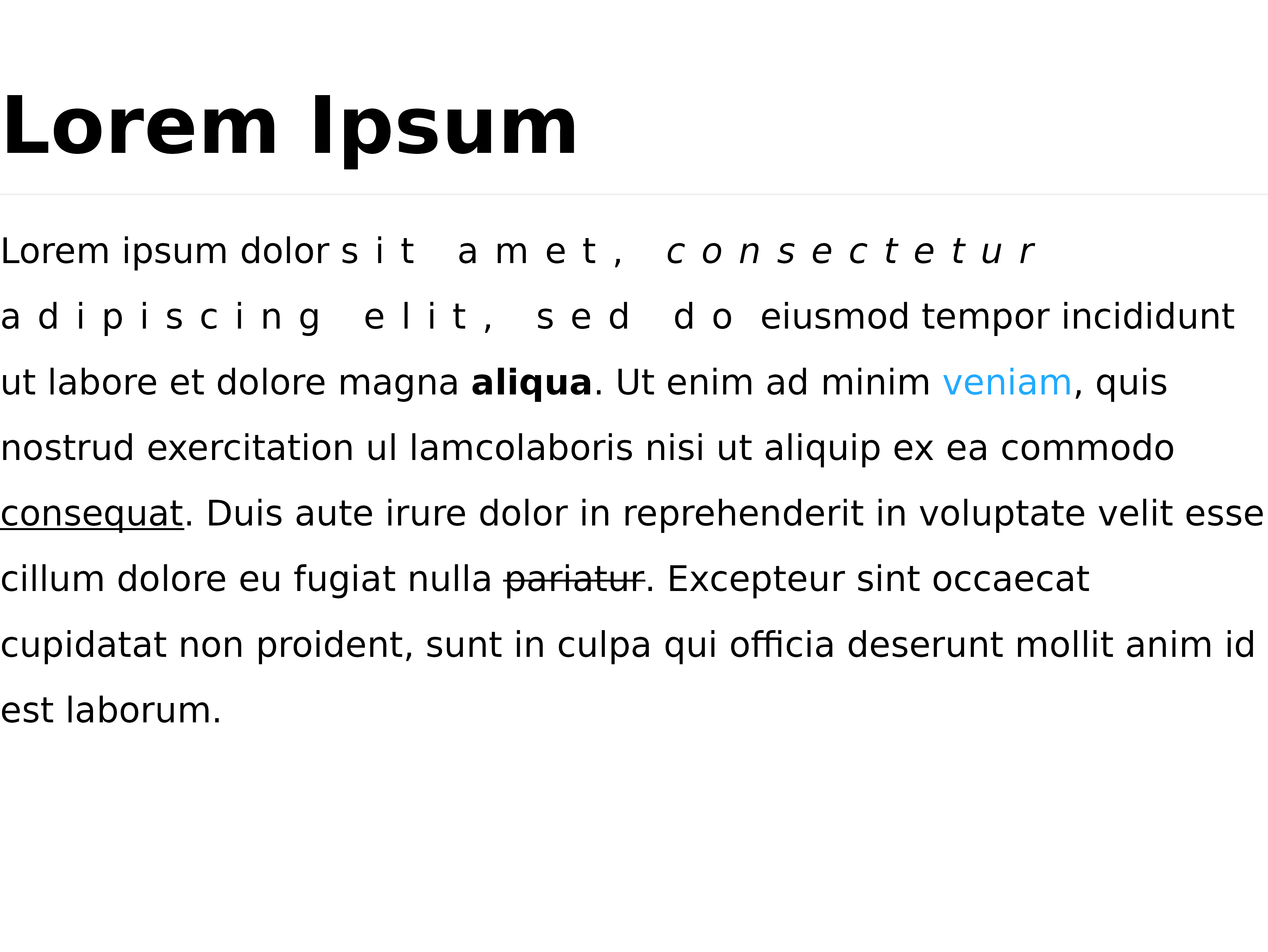
However, the main use will probably be to mix in italicized, bold, or colored fonts in labels, which marquee makes very easy
cars <- sub("(\\w+)", "{.red ***\\1***}", rownames(mtcars))
cars
#>  [1] "{.red ***Mazda***} RX4"
#>  [2] "{.red ***Mazda***} RX4 Wag"
#>  [3] "{.red ***Datsun***} 710"
#>  [4] "{.red ***Hornet***} 4 Drive"
#>  [5] "{.red ***Hornet***} Sportabout"
#>  [6] "{.red ***Valiant***}"
#>  [7] "{.red ***Duster***} 360"
#>  [8] "{.red ***Merc***} 240D"
#>  [9] "{.red ***Merc***} 230"
#> [10] "{.red ***Merc***} 280"
#> [11] "{.red ***Merc***} 280C"
#> [12] "{.red ***Merc***} 450SE"
#> [13] "{.red ***Merc***} 450SL"
#> [14] "{.red ***Merc***} 450SLC"
#> [15] "{.red ***Cadillac***} Fleetwood"
#> [16] "{.red ***Lincoln***} Continental"
#> [17] "{.red ***Chrysler***} Imperial"
#> [18] "{.red ***Fiat***} 128"
#> [19] "{.red ***Honda***} Civic"
#> [20] "{.red ***Toyota***} Corolla"
#> [21] "{.red ***Toyota***} Corona"
#> [22] "{.red ***Dodge***} Challenger"
#> [23] "{.red ***AMC***} Javelin"
#> [24] "{.red ***Camaro***} Z28"
#> [25] "{.red ***Pontiac***} Firebird"
#> [26] "{.red ***Fiat***} X1-9"
#> [27] "{.red ***Porsche***} 914-2"
#> [28] "{.red ***Lotus***} Europa"
#> [29] "{.red ***Ford***} Pantera L"
#> [30] "{.red ***Ferrari***} Dino"
#> [31] "{.red ***Maserati***} Bora"
#> [32] "{.red ***Volvo***} 142E"

ggplot(mtcars) + aes(disp, mpg, label = cars) +
  geom_marquee()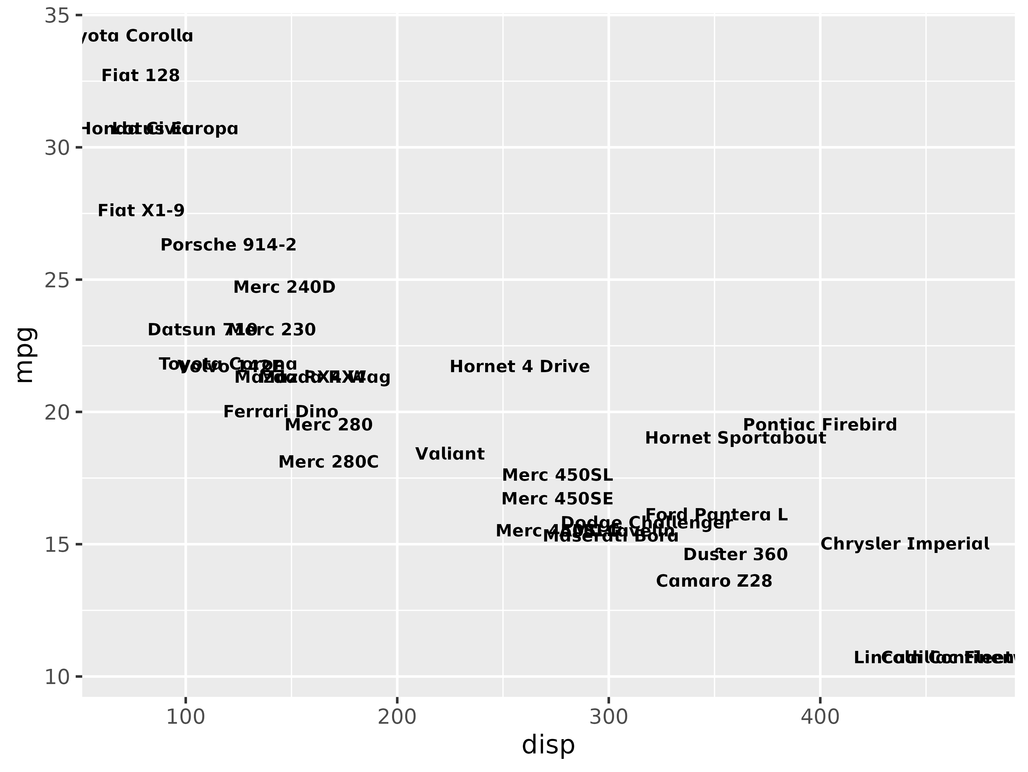
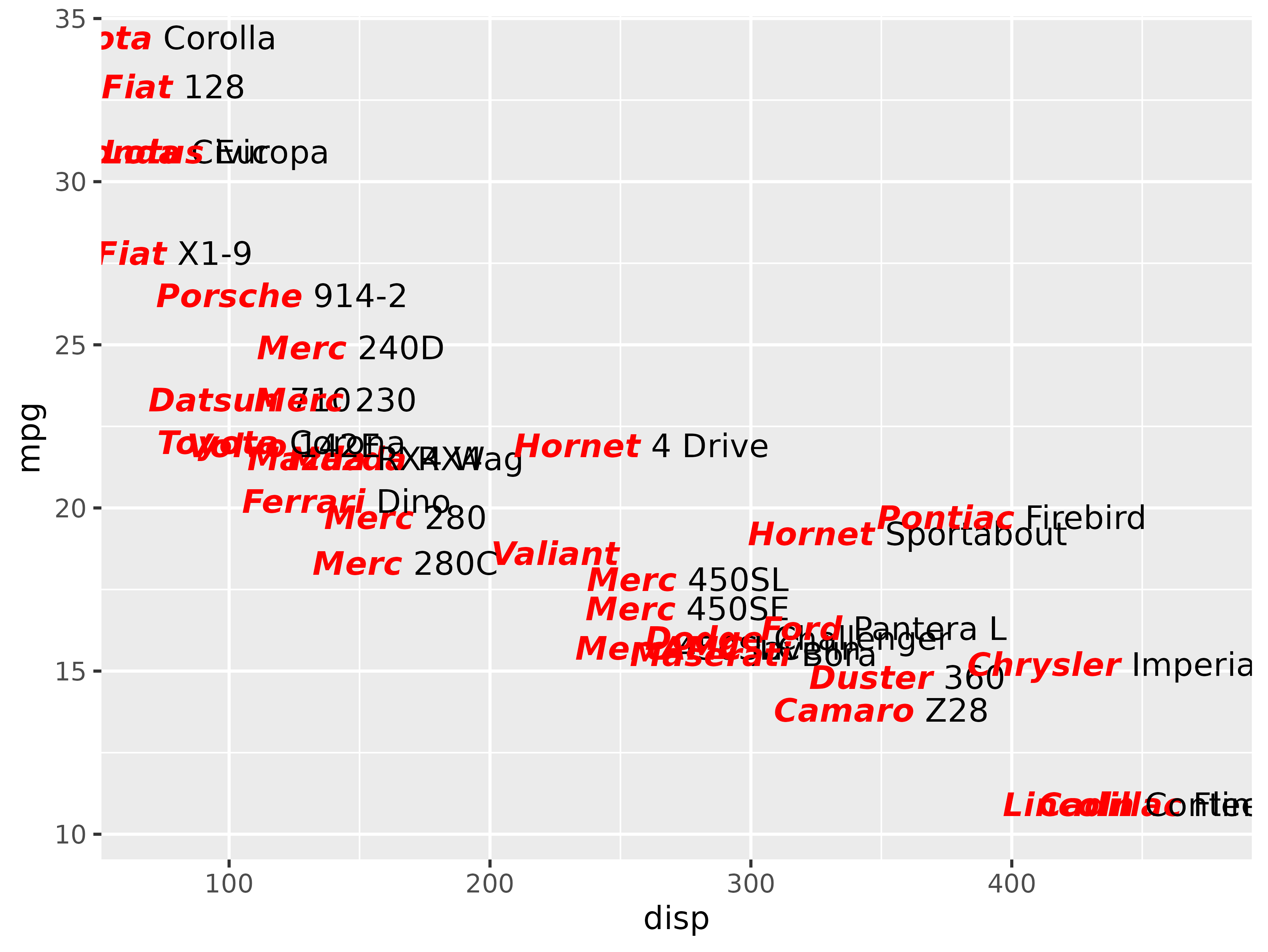
Another use of the geom, where rich text may come more into play, is in annotations. Let’s make a textbox style and add some lorem ipsum to our plot
text_box_style <- modify_style(
  classic_style(base_size = 2),
  "body",
  padding = skip_inherit(trbl(10)),
  border_radius = 3
)

ggplot(mtcars) + aes(disp, mpg, label = cars) +
  geom_marquee(size = 2) +
  annotate(GeomMarquee,
    label = md_text,
    x = 450,
    y = 35,
    style = text_box_style,
    size = 2,
    fill = "lightgrey",
    width = 0.3,
    hjust = "right",
    vjust = "top"
  )
The marquee element
Rich text in plotted text is probably limited in use, but when you
need it you really need it. Different from this is formatting of the
text that surrounds the plot. Here you tend to treat the text as rich
text and would want full control of the styling. Enter
element_marquee(), a drop-in substitute for
element_text() which will format and style any non-plotting
text.
ggplot(mtcars) + aes(disp, mpg, label = cars) +
  geom_marquee(size = 2) +
  ggtitle(md_text) +
  theme(plot.title = element_marquee(size = 9))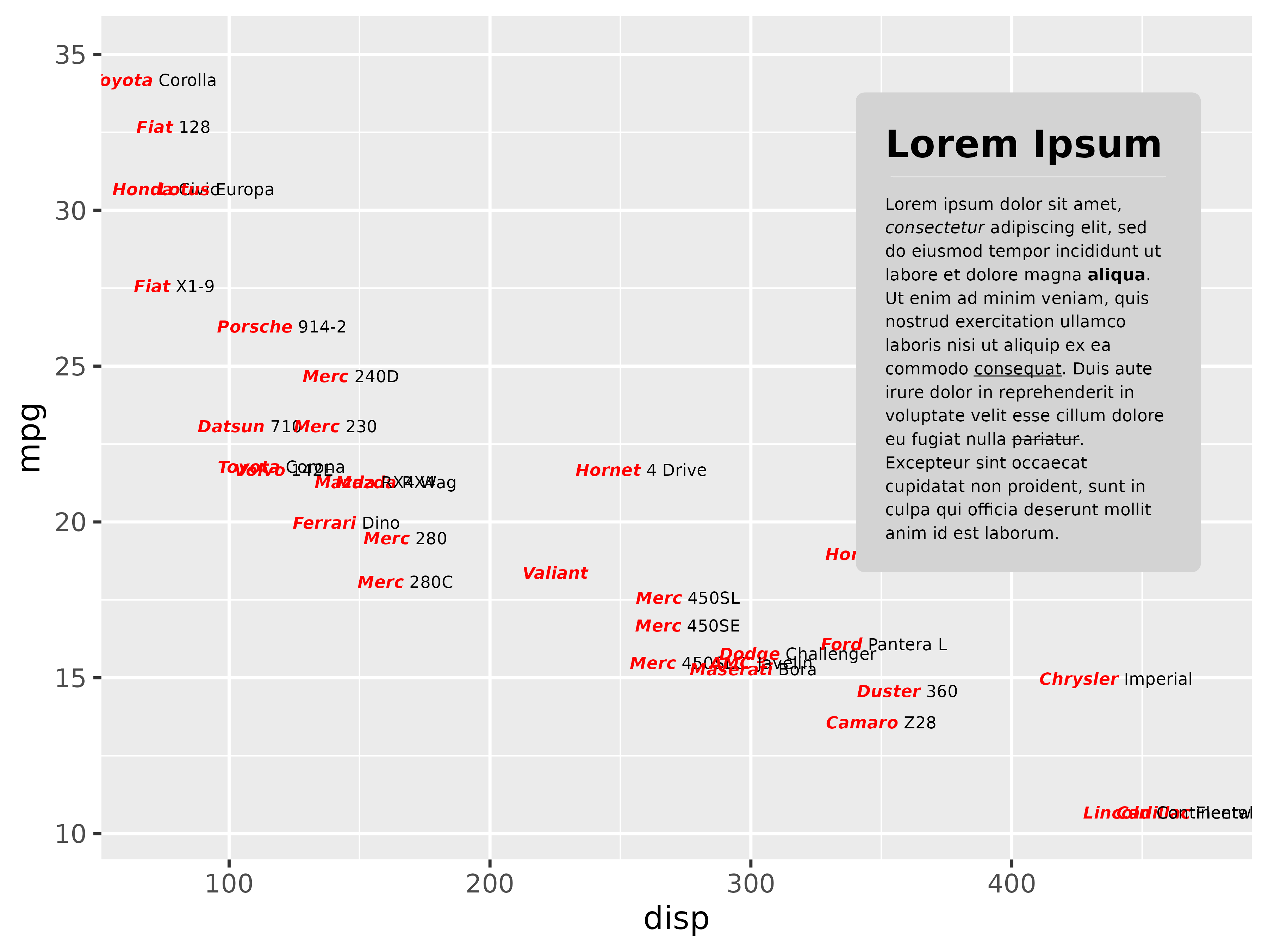
As can be seen, the defaults will let the text run for as long as it
needs without doing any text wrapping. This is because it makes
alignment behave in the same way as element_text().
However, if you have a lot of text like we do above, you certainly want
to turn on that feature. You do that by setting a width. 1
is equivalent to the width of the area the element occupies so that is a
natural value here, but you can set it to any grid::unit()
value you wish.
ggplot(mtcars) + aes(disp, mpg, label = cars) +
  geom_marquee(size = 2) +
  ggtitle(md_text) +
  theme(plot.title = element_marquee(size = 9, width = 1))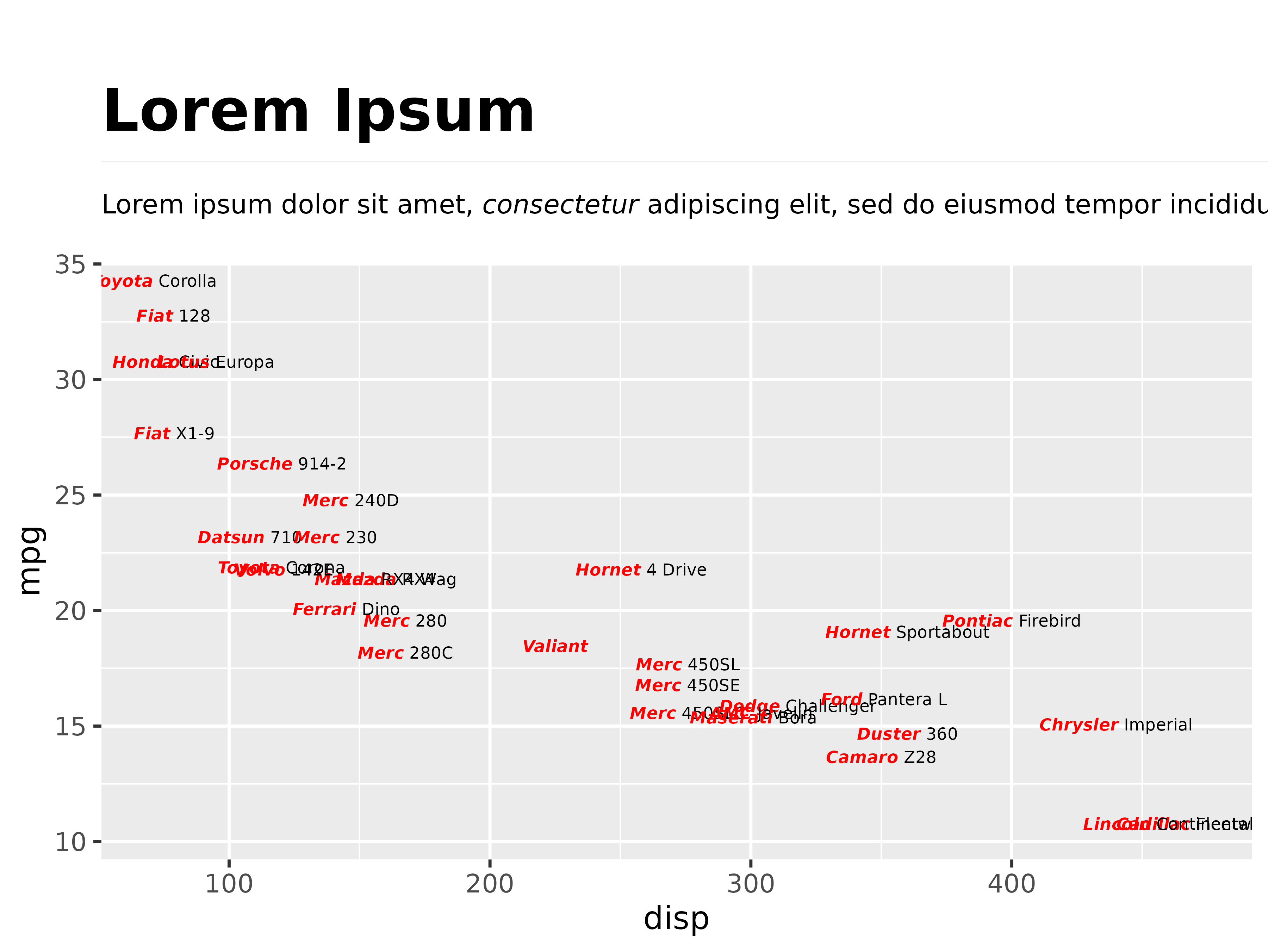
A bit about images
Markdown famously supports images through the ![]()
syntax. So does marquee of course (which means you can put images
everywhere in ggplot2 if you wish). Currently, there is support for PNG,
JPEG, and SVG, with the latter being responsive to resizing etc. The
images can reside online or on your computer — it all should “just
work”. If an image is placed inline it is sized to fit the height of
that line and adjusting the width to keep the correct aspect ratio. If
an image is placed by itself, it expands to fill the provided width,
width the height being calculated to match the aspect ratio of the
image.
md_text_fig <-
"# Lorem Ipsum 
Lorem ipsum dolor {.red sit amet, *consectetur* adipiscing elit, sed do} eiusmod tempor
incididunt ut labore et dolore magna **aliqua**. Ut enim ad minim {#2af veniam}, quis nostrud
exercitation ul lamcolaboris nisi ut aliquip ex ea commodo _consequat_. Duis aute irure dolor
in reprehenderit in voluptate velit esse cillum dolore eu fugiat nulla ~pariatur~. Excepteur
sint occaecat cupidatat non proident, sunt in culpa qui officia deserunt mollit anim id est
laborum."
grid.draw(marquee_grob(md_text_fig, classic_style()))
Compare that to
md_text_fig2 <-
"# Lorem Ipsum

Lorem ipsum dolor {.red sit amet, *consectetur* adipiscing elit, sed do} eiusmod tempor
incididunt ut labore et dolore magna **aliqua**. Ut enim ad minim {#2af veniam}, quis nostrud
exercitation ul lamcolaboris nisi ut aliquip ex ea commodo _consequat_. Duis aute irure dolor
in reprehenderit in voluptate velit esse cillum dolore eu fugiat nulla ~pariatur~. Excepteur
sint occaecat cupidatat non proident, sunt in culpa qui officia deserunt mollit anim id est
laborum."
grid.draw(marquee_grob(md_text_fig2, classic_style()))
However, marquee has a pretty unique trick up it’s sleeve compared to other markdown formats. It doesn’t just accept paths to images — it also accepts R graphic objects (currently grid grobs, ggplot2 plots and patchwork plots). It all works as you’d expect:
p <- ggplot(mtcars) +
geom_histogram(aes(x = gear))
md_text_plot <-
"# Lorem Ipsum

Lorem ipsum dolor {.red sit amet, *consectetur* adipiscing elit, sed do} eiusmod tempor
incididunt ut labore et dolore magna **aliqua**. Ut enim ad minim {#2af veniam}, quis nostrud
exercitation ul lamcolaboris nisi ut aliquip ex ea commodo _consequat_. Duis aute irure dolor
in reprehenderit in voluptate velit esse cillum dolore eu fugiat nulla ~pariatur~. Excepteur
sint occaecat cupidatat non proident, sunt in culpa qui officia deserunt mollit anim id est
laborum."
grid.draw(marquee_grob(md_text_plot, classic_style()))
#> `stat_bin()` using `bins = 30`. Pick better value `binwidth`.
A bit about tables
The table markdown syntax is not supported in marquee. However, you can still include tables in marquee, and with much more styling support than standard markdown table syntax provide. This magic is an extension of what was talked about above. More to the point, gt table objects are recognized as valid objects in the image tag path and can thus be included directly in the output. We show the power here with a table specification taken from the gt introduction:
library(gt)
airquality_m <- airquality[1:10, ]
airquality_m$Year <- 1973L
table <- gt(airquality_m)
table <- tab_header(table,
  title = "New York Air Quality Measurements",
  subtitle = "Daily measurements in New York City (May 1-10, 1973)"
)
table <- tab_spanner(table,
  label = "Time",
  columns = c(Year, Month, Day)
)
table <- tab_spanner(table,
  label = "Measurement",
  columns = c(Ozone, Solar.R, Wind, Temp)
)
md_text_table <-
"# Lorem Ipsum
Below we have a table created with gt

*Such tables, much cells*"
grid.draw(marquee_grob(md_text_table, classic_style()))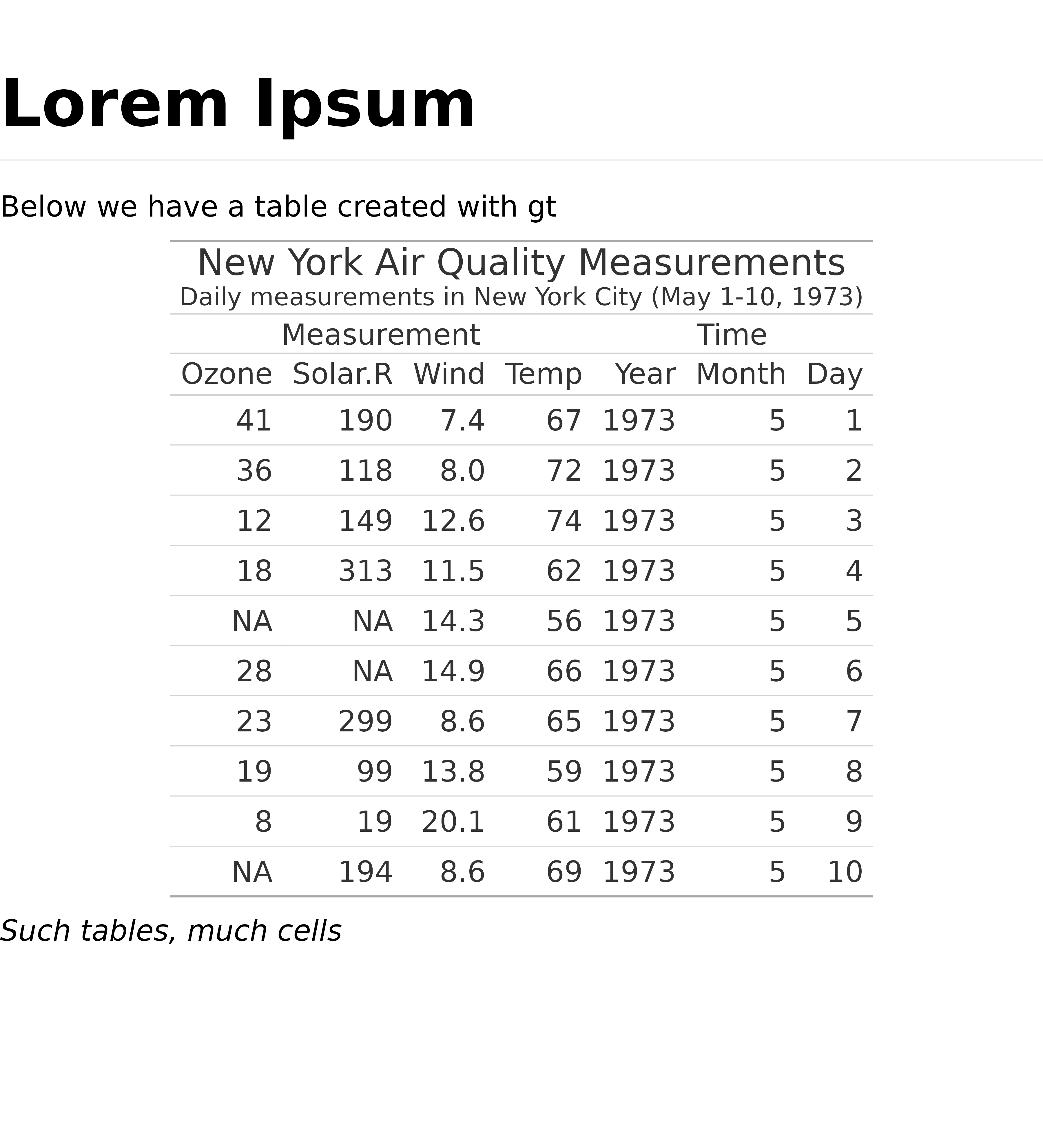
The support is still somewhat experimental as gt-to-grob conversion is getting build out. Some gt features rely on HTML formatting still and will end up looking weird, but standard table inclusion works as expected.
